First Things First

This being my debut blog post, I thought I should start with my motivation for creating the blog. I entered the world of rendering pretty late into my undergraduate degree, but what originally drew me in was all the amazing rendering projects people have shared online. I've been working on my own personal renderer Dino for a few years now, which was inspired by these blogs and ultimately led to my decision to pursue rendering as a career. The purpose of this blog is to motivate me to keep working on my own projects, and also to give a bit back to the online world and maybe inspire someone else to enter this exciting field.

While I won't be retroactively posting about how I set up the basics (there are plenty of online resources which cover these topics¹), I would like to cover more advanced topics or those which I think could be helpful for beginners but don't have much online coverage.

Now, on to the actual post.

Uniform

pmj02bn

Monte Carlo integration is a key technique required for modern rendering. The classic example of Monte Carlo integration is a simple algorithm which estimates \(\pi\) by generating random points on a square and counting the number of points which happen to fall inside a circle embedded in the square. Conceptually, this is exactly how modern rendering works, only instead of integrating the area of a circle we are solving a much more complex lighting integral. Consider the Rendering Equation ².

\[L_o(\bm\omega_o) = L_e(\bm\omega_o) + \int\limits_\Omega L_i(\bm\omega_i) f(\bm\omega_o, \bm\omega_i) |cos\theta_i| d\bm\omega_i\]

Everything within the integral is solved with a Monte Carlo estimator. The \(|cos\theta_i|\) term can usually be solved analytically, but the BRDF \(f\) and the incident lighting \(L_i\) are often both too complex for analytic integration. The full product \(L_i(\bm\omega_i) f(\bm\omega_o, \bm\omega_i) |cos\theta_i|\) just complicates things further, making Monte Carlo integration the only choice in non-trivial cases. Since this is still 2D integration (we are integrating over \(\Omega\), the 2D surface of the unit hemisphere) we still generate point samples on the 2D unit square \([0, 1)^2\), but warp them as needed for whatever sampling method we're using (BRDF importance sampling, next event estimation, etc.). A naive renderer will use uniformly random 2D samples, but it turns out there is a much better way.

Generating a Strong Sample Pattern

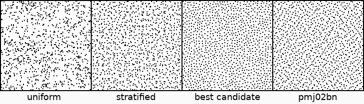
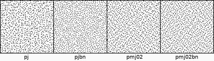
The image above shows a brief selection of sample patterns that can be used for rendering. Random samples tend to cluster together in some places and leave holes in other places which results in slow convergence. Stratified or "jittered" sampling aims to correct this problem by constraining each random sample to a unique cell of a grid, which spreads them more evenly across the square and improves convergence. Best candidate sampling solves the clustering problem by generating only points which are as far as possible from any other point in the sequence, producing an interesting "blue noise" pattern which also improves convergence over uniformly random sampling.

The final pattern's full name is "progressive multi-jittered (0, 2) sequences with blue noise properties", or pmj02bn for short (though this is still a mouthful). It was introduced fairly recently by some folks at Pixar in the 2018 paper Progressive Multi-Jittered Sample Sequences (I'll just call it the PMJ paper). It doesn't look particularly special compared to stratified or best candidate samples, but it is carefully designed to maximize convergence and have a number of useful properties, which is why I chose it as Dino³'s sample pattern. I'll cover a few of these properties below, borrowing a few graphics from the original paper.

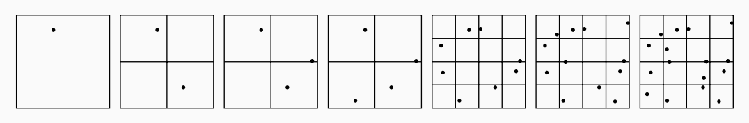
Property 1: Progressiveness

First, pmj02bn is a progressive sequence. Many sample patterns such as stratified or Correlated Multi-Jitter require you to know how many samples you want to use before rendering even begins and have higher error if you end up using a different number of samples. By contrast, a progressive sequence converges consistently regardless of how many samples you decide to use. This property turns out to be very important in features such as adaptive sampling and interactive rendering, where you don't know how many samples a pixel will get beforehand. In the case of the progressive sequences introduced in the PMJ paper (including pmj02bn) samples are placed in a continuously-subdivided grid in a very specific pattern which spreads them out very evenly.

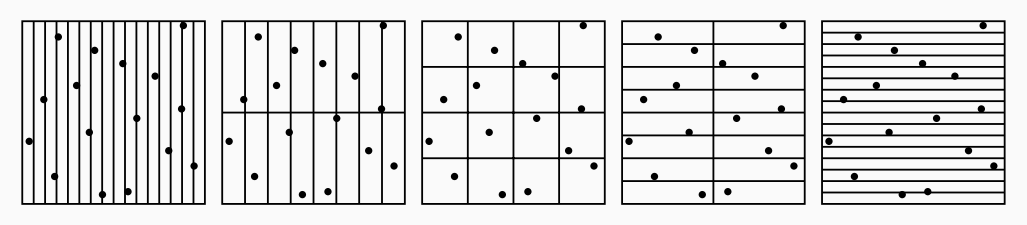
Property 2: (0, 2) Sequence

The second useful property of pmj02bn is that it is a (0, 2) sequence. As with stratified sampling, a (0, 2) sequence guarantees each sample will fall within a different grid cell, but it makes this guarantee for several grids of various dimensions rather than just one. By stratifying across all of these cell shapes, or base 2 elementary intervals, samples are more strictly structured which leads to better convergence and greater resilience in cases of high warping. This resilience to warping turns out to be important for rendering since we tend to squash and stretch our samples quite a bit to fit our needs, for example sampling a rectangular light source which is very tall and narrow.

Property 3: Blue Noise

The last property I want to mention is the "blue noise" or bn portion of pmj02bn. I've already briefly mentioned that the best candidate method generates a "blue noise" pattern which spreads samples out more evenly. It does this by generating multiple uniformly random candidate samples, then selecting the one which is farthest from any other sample previously added to the sequence. pmj02bn does exactly the same thing, but generates candidates according to the progressive and (0, 2) constraints. The samples are thus spread out a bit more, but due to the strict constraints they aren't quite as well-spaced as they could be. The paper actually mentions it comes down to a choice between the better convergence of pmj02bn and the more visually pleasing patterns generated by removing the (0, 2) constraints.

Efficient Sample Generation

The PMJ paper comes with a very helpful supplemental document which includes pseudocode for generating any of the several progressive sequences introduced by the paper. Unfortunately, this pseudocode works by generating random samples according to the progressive pattern I mentioned above, then checking all the (0, 2) constraints before accepting them. This is fine for a small number of samples with coarse elementary intervals, but when many thousands of samples are required the (0, 2) constraints make it difficult to find an acceptable sample. Thankfully, Matt Pharr published an improved sample generation technique which very efficiently produces random samples which already satisfy these (0, 2) constraints, leading to a huge improvement in speed for generating pmj02bn samples.

Rendering with Strong Samples

Using strong 2D samples in a renderer is conceptually straightforward, but you have to be careful or similarities in the patterns will result in correlation artifacts or noise that never really converges. The final method I settled on is based on descriptions of Pixar's RenderMan and also Blender's awesome open-source Cycles renderer.

Sampling in Dino

According to the PMJ paper, RenderMan pre-generates several hundred pmj02bn sequences which each contain only the first 4,096 samples. They hash the pixel index and ray depth to a specific sequence so each stochastic event which occurs when constructing each path uses an independent sequence. Dino is slightly different. I sometimes use more than 4,096 samples for a very clean render in a complex scene (a better integrator or any sort of denoising will be a better choice in the future), so I implemented Matt Pharr's improved sample generator and pre-generate 32 sequences of 16,384 samples which are used for every render. The generator proposed by the PMJ paper would do this in several minutes, but the improved generator gives me results almost immediately! I then distribute the samples from these 32 channels as needed during rendering.

There are several stochastic events in a typical path tracer which consume 2D samples, and these may vary based on what sort of integrator you're using or techniques you've implemented. In the case of Dino's forward path tracing integrator, there are four places which require 2D samples: pixel filter sampling, lens area sampling (for depth of field), BSDF sampling, and light source sampling. Pixel filter and lens area sampling each require only one 2D sample per path, so only 2 of the 32 channels are required for them. BSDF and light samples are different in that they are required each bounce, so a theoretically infinite number of channels are required for both. I settle for using only 8 channels for each, then wrapping when a path gets too large. This is very unlikely to cause correlation issues in most scenes, but it is possible, eg. if a path hits a diffuse surface then bounces off 7 mirrors before hitting another diffuse surface. A production renderer should avoid this and probably shuffle channels with hashing like RenderMan does.

RenderMan decorrelates pixels by including the pixel index in the hash which selects a sequence. By contrast, Dino just uses the same channels for each pixel and decorrelates by using random Cranley-Patterson rotations for each pixel/channel pair. This is possibly not as effective as the hashing RenderMan does, but will end up being useful in the future!

Correlation Woes

After implementing everything as described above, I was excited to see the fruits of my labor. Unfortunately, my first renders with these progressive patterns ended up producing strange noise in areas with a lot of indirect lighting, and also artifacting around the edges of objects. This is immediately identifiable as correlation issues: indirect lighting requires chaining several BSDF samples, and edge artifacting can indicate correlation between pixel filter samples and BSDF samples.

I thought at first that my implementation was incorrect, but I eventually discovered that shuffling the sequences after generation produced the nice, clean renders I was looking for. It turns out that all of the progressive patterns introduced in the PMJ paper actually cause correlation issues if chained together as in a path tracer unless you shuffle things around a bit. My first solution for this involved shuffling an exponentially-increasing portion of the samples as they were generated, which removed the correlations but also destroyed a lot of the progressiveness of the patterns. Thankfully, in my search for a better solution, I found that Blender's Cycles renderer recently implemented pmj02bn. Their code solves the correlation issue by shuffling every chunk of 16 samples as a post-processing step after the whole sequence has been generated. This preserves progressiveness but also completely removes the correlation artifacts. Score!

Original

Shuffled

Results

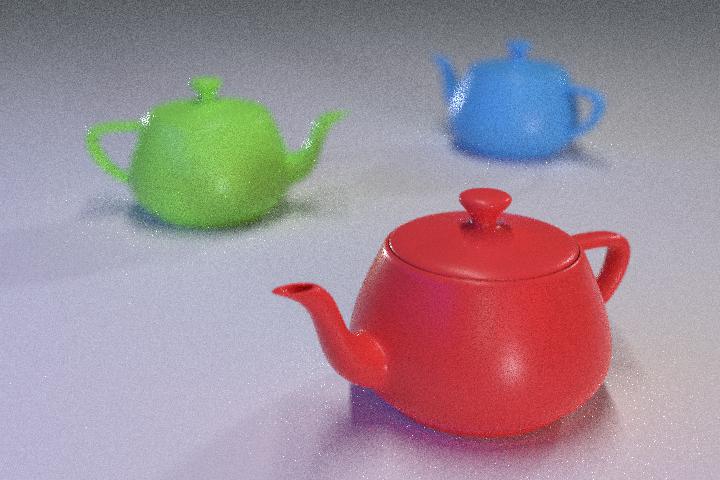
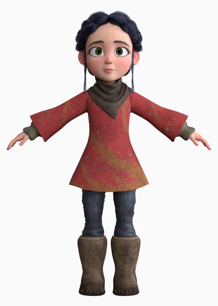
Finally, I wanted to highlight the improvements I saw in Dino by switching from uniform to pmj02bn with some higher-quality assets than simple teapots and dragons. One of my current goals with Dino is to render a production-quality animation with believable characters. It's a big undertaking, and having an efficient renderer is super important when you're trying to render many frames of highly complex scenes.

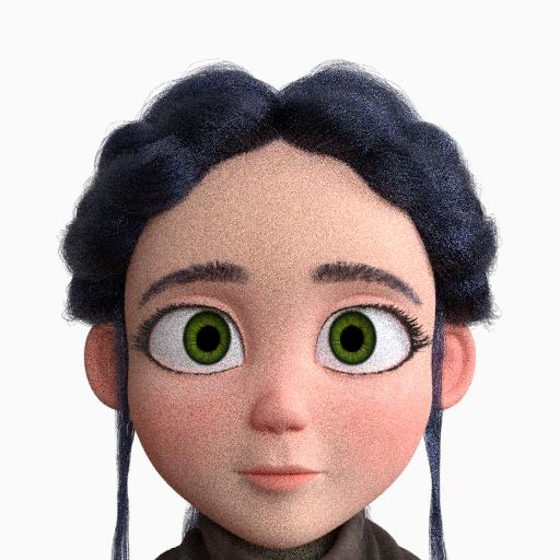
Usually it's difficult just to find production data available for personal use. Thankfully, the Blender Foundation has been producing what they call Open Movies where they make a short film and then release the project files (characters, props, entire shots—everything) to the public. It requires a monthly subscription to access most of the project files but you get project assets and animations from a ton of their short films. Below are some results using the main character from the Blender short film Spring.

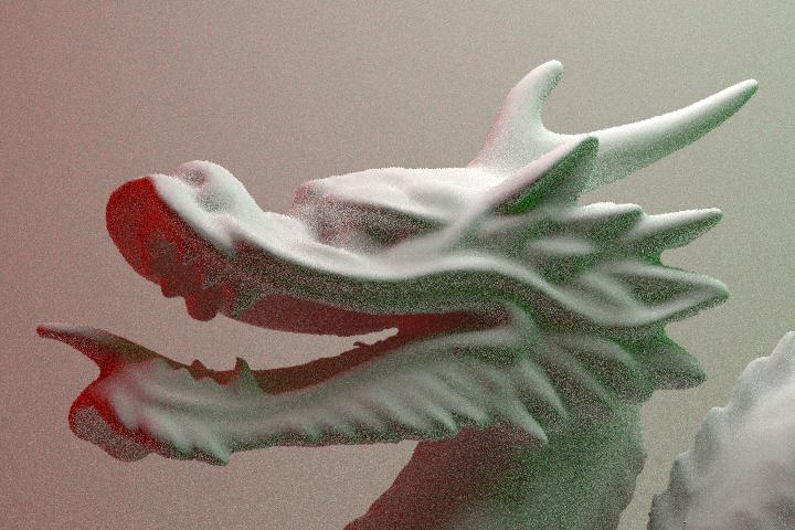
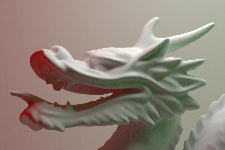
Uniform

pmj02bn

The benefit of improved sampling is pretty clear. Spring's skin shows the largest improvement, which somewhat surprised me since Dino currently still uses uniform random samples for Monte Carlo subsurface scattering which the skin uses. Unsurprisingly, the hair shows the least improvement since much of the color of hair comes from indirect bounces⁴ which have diminishing returns even with a good sample pattern. If we zoom into Spring's head the skin improvement is even clearer and we can see that the hair actually is slightly improved.

Uniform

pmj02bn

Conclusion

I've been using simpler sample patterns for a while, but held off using more robust sequences because it seemed much more interesting to implement new materials or effects. But sampling is an interesting topic in its own right, and faster convergence mean you can have more complex scenes and faster turnaround during development which is a big win.

I'm currently working on some related features including adaptive sampling, which I'll post about in the future. In my tests, the improvements I achieved on Spring's skin and clothes correspond to about a 3× speed improvement switching from uniform to pmj02bn, which seems great because these are the largest parts of the character. Unfortunately, this improvement is wasted now because the hair is the bottleneck which drives the required number of samples per pixel and thus render time. With adaptive sampling, Dino will be able to take advantage of this improvement since the number of samples per pixel will no longer be fixed to whatever feature is causing the bottleneck.