In my last post, I talked about how Dino handles sampling. I mentioned that I chose Cranley-Patterson rotations¹ over hashing to decorrelate pixels even though they are probably less effective at reducing noise². I made this decision because I wanted to play with an interesting rendering technique from a 2018 paper entitled Blue-noise Dithered Sampling which takes advantage of correlations between pixels to reduce perceptual error. I'll talk about exactly what that means, and render some results with my personal renderer Dino.

Correlation is Bad

I previously discussed some correlation issues I ran into while implementing better sampling for Dino which manifested as noise and edge artifacts. These issues appeared because the sample patterns I used were structurally too similar to each other and ended up constructing similar light paths multiple times while avoiding others. The solution was to randomly shuffle parts of the sequence to remove the correlations, letting the renderer explore all light paths while maintaining the strong sampling properties.

The correlation we're considering in this post is of a slightly different nature. Rather than considering similar paths within a pixel, we're now interested in similar paths among nearby pixels. If two nearby pixels are correlated, they generate similar paths and thus their results will likely be similar. The only differences come from their slightly different pixel locations, though this can cause a butterfly effect leading to very different outputs depending on the scene being rendered.

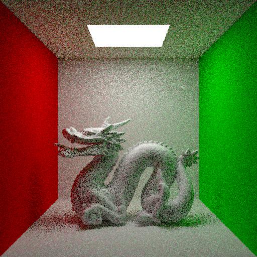
It's actually pretty easy to see pixel correlations in action. I'm going to render the same simple scene several times, only changing the Cranley-Patterson rotations. For the first few renders, next event estimation is disabled so we can focus on how pixel correlations affect just BSDF sampling (this just makes the correlations easier to see). First, let's start with a reference image so we know what the scene should look like.

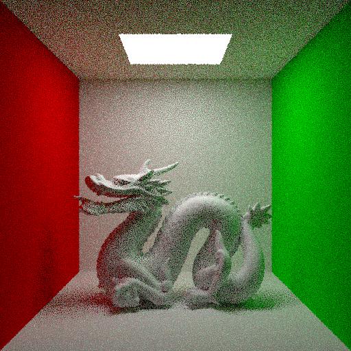
Now, let's look at the same scene, rendered with only 4 samples per pixel and standard, uniformly random Cranley-Patterson rotations. We should get the gist of what it should look like, but the image will be quite noisy, especially since next event estimation is disabled.

Now we're going to do something a little strange. Instead of trying to de-correlate pixels, we're going to try to correlate them as much as possible. Since the only mechanism in place right now which decorrelates pixels is the random per-pixel Cranley-Patterson rotations, let's see what happens when we set them all to the same 2D vector, specifically \((0, 0)\).

Wow. It looks terrible. What happened?

It's actually not too difficult to understand why this happens. Since we're feeding the same 2D sample to the BSDF sampling function in every pixel, all paths which bounce off a flat, diffuse surface like a wall end up going in exactly the same direction. The largest of the blocky patches on the walls are where the paths bounce just once, and the bounce direction happens to line up with the top light source. The smaller patches are from further bouncing, and much of the noise comes from the dragon which decorrelates things a bit with its curved surface since light no longer bounces in quite the same direction.

It's important to note that although this image looks really bad compared to the first noisy render, images produced with either method will have exactly the same error when compared against the reference image, at least on average. In fact, given enough time the constant-rotation image will converge to the reference just as the random-rotation image would! Don't believe me? See for yourself below.

Trippy.

But even if rendering like this is technically unbiased, it's pretty clear that you would never use something like this for anything practical.

Correlation is Not Always Bad

So far, I've shown how correlation is generally best avoided during rendering, but a key insight of the Blue-noise Dithered Sampling paper is that correlation can actually be helpful—if you know how to use it. As we've seen above, we have some control over pixel correlations with Cranley-Patterson rotations, we just don't know of any way to pick rotations which is better than uniformly random.

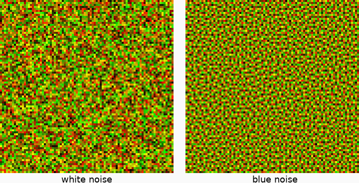
Enter blue noise. If we pick uniformly random 2D vectors for each pixel, we end up generating uncorrelated white noise, which can looks sort of chunky. By contrast, blue noise cuts out all of the low-frequency chunkiness, leaving only high-frequency noise and tends to look more pleasant and uniform than white noise. The Blue-noise Dithered Sampling paper introduces a very simple algorithm to create blue noise textures that we can use for Cranley-Patterson rotations by optimizing an energy function on the image. Optimization can sometimes be finicky to implement and use, but the basic algorithm to generate a \(d\)-dimensional blue noise texture is very straightforward:

1. Generate a white noise texture of random vectors \(\in [0, 1)^d\).
2. Pick 2 random pixels, then swap them if doing so reduces the energy function (see paper).
3. Repeat step 2 until a blue noise pattern emerges.

I told you it was easy! The only issue is that the energy is technically a function over an infinite number of points, but the contributions drop off with distance so using a \(9\times9\) window around the target pixels is sufficient. Here's all the code you need to generate a 2D blue noise texture³:

float energy(const std::vector<glm::vec2>& buffer, glm::ivec2 a)
{
    int ia = a.y * BLUE_NOISE_DIM + a.x;

    // Loop over 9x9 region around target pixel.
    float totalEnergy = 0.0f;
    for (int dy = -4; dy <= 4; dy++) {
        for (int dx = -4; dx <= 4; dx++) {
            if (dx == 0 && dy == 0) continue;

            // Find coordinates of second pixel, wrapping if necessary.
            glm::ivec2 b(
                (a.x + dx + BLUE_NOISE_DIM) % BLUE_NOISE_DIM,
                (a.y + dy + BLUE_NOISE_DIM) % BLUE_NOISE_DIM);
            int ib = b.y * BLUE_NOISE_DIM + b.x;

            // Add to total energy using energy function from the paper.
            // This is the 2D case: d = 2 (optimized out)
            // Use recommended parameters:
            //     sigma_i = 2.1
            //     sigma_s = 1.0 (optimized out)
            totalEnergy += std::exp(
                -glm::length2(glm::vec2(dx, dy)) / (2.1f * 2.1f)
                - glm::distance(buffer[ia], buffer[ib]));
        }
    }

    return totalEnergy;
}

void minimizeEnergy(std::vector<glm::vec2>& buffer)
{
    // Try to swap pixels for many iterations.
    for (int i = 0; i < NUM_ITERATIONS; i++) {

        // Select two random pixels.
        glm::ivec2 a(randomu() % BLUE_NOISE_DIM, randomu() % BLUE_NOISE_DIM);
        glm::ivec2 b(randomu() % BLUE_NOISE_DIM, randomu() % BLUE_NOISE_DIM);
        if (a == b) continue;

        // Find pixel indices in buffer.
        int ia = a.y * BLUE_NOISE_DIM + a.x;
        int ib = b.y * BLUE_NOISE_DIM + b.x;

        // Find energy before and after swapping pixels.
        float startEnergy = energy(buffer, a) + energy(buffer, b);
        std::swap(buffer[ia], buffer[ib]);
        float endEnergy = energy(buffer, a) + energy(buffer, b);

        // If the energy was lower before the swap, then swap back.
        if (startEnergy < endEnergy) {
            std::swap(buffer[ia], buffer[ib]);
        }
    }
}

std::vector<glm::vec2> generateBlueNoise()
{
    // Initialize the texture with white noise.
    std::vector<glm::vec2> buffer(BLUE_NOISE_DIM * BLUE_NOISE_DIM);
    for (glm::vec2& val : buffer) {
        val = glm::vec2(randomf(), randomf());
    }

    // Minimize energy and return the resulting blue noise texture.
    minimizeEnergy(buffer);
    return buffer;
}

Dino uses the paper's recommended texture size (\(128\times128\), so BLUE_NOISE_DIM = 128), and minimizes the energy for about 4,000,000 iterations⁴. Results are shown below.

All we need to do now is plug these 2D blue noise vectors in as Cranley-Patterson rotations instead of using uncorrelated, uniformly random rotations. We'll need a unique blue noise texture for each stochastic event, or, in Dino's case, a unique texture for each of the 32 sample channels. In these last renders, I'll turn next event estimation back on.

Uncorrelated

Blue Noise

Uncorrelated

Blue Noise

There is a small, but definitely noticable improvement! Although the error is technically unchanged, the visible blue noise patterns make the renders appear more converged⁵. But does this hold up when we use slightly more complex shapes, materials, and lighting?

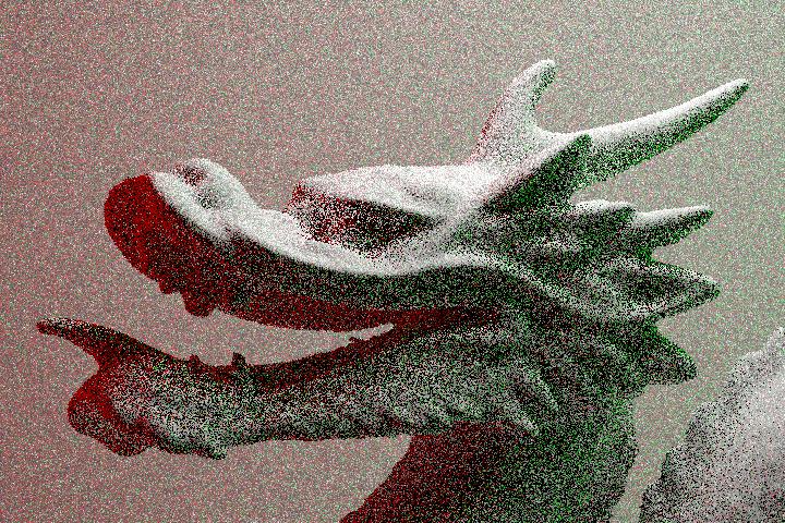
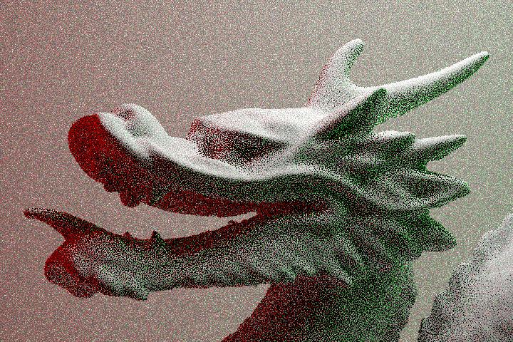
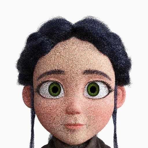Uncorrelated

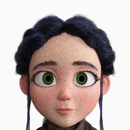Blue Noise

This is an even bigger improvement than with the dragons! Unfortunately, blue noise dithering can't really help out when a lot of indirect bounces are needed as with Spring's hair. Also, the benefits tend to disappear when you try to use more than just a few samples per pixel. Still, this can be a useful technique eg. for cleaning up early progressive renders, especially since denoisers can perform better when blue noise patterns are used.

Conclusion

I was very satisfied with the results I got for blue noise dithering with low sample counts, but it would have been nice to keep these patterns for higher sample counts so it could actually be useful for cleaner renders. Thankfully this technique is very new and there's been some interest in improving on it. Notably, Heitz et al. introduced two improvements last year. The first technique introduces a way to do blue noise dithered sampling without Cranley-Patterson rotations, somewhat improving results especially when more samples are used. The second technique introduces blue noise patterns not from pixel-local decisions, but through adaptively sorting a neighborhood of pixel samples based on their expected output.

I think the adaptive sorting is particularly interesting and I'd like to try implementing it at some point. However, since I also want to implement adaptive sampling, I wonder how this sorting can work if not all pixels have the same sample count.